Home > Knowledge Base > Statistical Analysis > Central Limit Theorem

Central Limit Theorem

Published by Alaxendra Bets at November 18th, 2025 , Revised On November 18, 2025

Let’s say that you want to predict the average exam score of an entire university based on a few randomly chosen classes. Or maybe you want to analyse customer ratings to estimate the true satisfaction level of a large population.

In both cases, you are working with samples, which are smaller portions of a much larger dataset. But how can you trust that your sample average represents the actual population average?

That is where the Central Limit Theorem (CLT) steps in.

What Is The Central Limit Theorem

The Central Limit Theorem (CLT) states that when you take a large number of random samples from any population, regardless of its shape (skewed, uniform, or otherwise), the distribution of the sample means will tend to approach a normal distribution as the sample size increases.

Mathematically, this means that even if your population data is irregular or asymmetric, the average of many random samples will still form a bell curve centred around the true population mean.

Think of what happens when you are rolling a single die. The results are uniform, each number from 1 to 6 equally likely. But if you roll many dice and take their average, that average will start to cluster around the middle (3.5). Do this enough times, and your distribution of averages will look almost perfectly normal.

This simple yet powerful principle allows statisticians to use normal probability models to estimate population parameters, even when the original data are not normal.

Want Custom Dissertation Topic?

Our writers are ready to deliver multiple custom topic suggestions straight to your email that aligns
with your requirements and preferences:

Original Topic Selection Criteria
Ethics Of Sensitive Topics
Manageable Time Frame Topics

Sample Dissertation Whatsapp Us Order Now

Key Assumptions And Conditions Of The Central Limit Theorem

Before applying the Central Limit Theorem (CLT), it’s essential to understand its core assumptions and conditions.

1. Random Sampling

The first condition for the Central Limit Theorem is random sampling.

Each sample must be chosen randomly from the population to avoid bias. If samples are not random, the resulting sample means may not accurately represent the population, leading to distorted conclusions.

Tip: In research, using proper randomisation methods (like random number generators or random assignment) ensures this assumption is met.

2. Sample Size and Independence

The sample size plays a major role in how quickly the sampling distribution approaches normality.

For many practical purposes, a sample size of 30 or more is often sufficient (though this can vary).
Samples must also be independent, which means that the selection of one sample should not influence another.

Independence ensures that each data point contributes uniquely to the overall analysis, maintaining statistical validity.

3. Population Variance and Shape

The Central Limit Theorem applies regardless of the population’s shape, whether it is uniform, skewed, or irregular. However, it assumes that the population has a finite variance.

If the population variance is infinite (as in certain heavy-tailed distributions), the theorem does not hold.

Heavily skewed distributions may require larger sample sizes.
Normal populations converge faster under CLT conditions.

What happens when these conditions are not met?

Meeting these assumptions ensures that your sample means follow a normal distribution, even when the population does not. This is crucial for accurate hypothesis testing, confidence intervals, and other inferential techniques.

If any condition is violated, such as biased sampling or dependent data, the Central Limit Theorem’s results may not be valid.

Mathematical Representation And Formula

The Central Limit Theorem formula gives a clear mathematical view of how sample means behave when random samples are drawn repeatedly from a population. It forms the basis for most inferential statistical calculations.

According to the Central Limit Theorem:

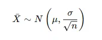
This equation shows that the sampling distribution of the sample mean (X) is approximately normal, with:

Mean (μ) is equal to the population mean
Standard deviation (σ/√n), also called the standard error of the mean

Symbol	Meaning	Description
μ	Population Mean	The true average value of the entire population.
σ	Population Standard Deviation	Measures how spread out the data is within the population.
n	Sample Size	The number of observations in each sample.
X	Sample Mean	The average value calculated from a random sample.
N(μ, σ/√n)	Normal Distribution	Indicates that the sample means form a normal distribution centred at μ.

What the formula tells us

As n increases, the standard error (σ/√n) decreases, which means that the sample mean becomes a more accurate estimate of the population mean.
Even if the population distribution is not normal, the mean distribution of large random samples will approximate normality.
This allows statisticians to apply z-scores, confidence intervals, and hypothesis tests using normal probability theory.

Practical Example

Imagine the average height (μ) of all students in a university is 170 cm with a population standard deviation (σ) of 10 cm.

If you take random samples of n = 25 students, then:

Standard Error = 10 / 25 = 2

This means the sample means (average heights from each group of 25 students) will follow a normal distribution N(170, 2), centred at 170 cm with less variation than the population itself.

Central Limit Theorem Examples

Here are some simple and practical examples of the Central Limit Theorem that show how it works in everyday scenarios.

1. Example in Education: Average Exam Scores

Imagine a university wants to estimate the average score of all students. Instead of checking every student’s result, the researcher takes multiple random samples of students and calculates the average score for each group.

As the number of samples increases, the distribution of those average scores becomes approximately normal, even if the original scores were skewed.
This helps the university make reliable predictions about student performance without testing the entire population.

2. Example in Business: Customer Ratings

Suppose an online store collects customer ratings from thousands of buyers.

If you take several random samples of these ratings and compute their averages:

Each group might differ slightly, but the average of averages will form a bell-shaped (normal) curve.
This allows marketers to estimate overall satisfaction and understand customer trends more accurately.

3. Example in Manufacturing: Quality Control

A company producing light bulbs wants to ensure a consistent product lifespan.

Instead of testing every bulb, they take random samples from each batch and record their average burn time.

According to the CLT, these sample averages will follow a normal distribution.
This helps identify whether a batch deviates from the expected lifespan, ensuring quality assurance and process stability.

4. Example in Healthcare: Average Blood Pressure

Researchers studying the average blood pressure of adults do not test everyone.

They take multiple random samples of patients from different regions.

As the sample size grows, the distribution of sample means becomes normal.
This enables the use of confidence intervals and hypothesis testing to make inferences about the entire population.

Central Limit Theorem Vs Law Of Large Numbers

Both the Central Limit Theorem (CLT) and the Law of Large Numbers (LLN) are essential principles in probability and statistics.

While they often appear together, they explain different aspects of sampling behaviour.

	Central Limit Theorem (CLT)	Law of Large Numbers (LLN)
Definition	States that the distribution of sample means approaches a normal distribution as the sample size increases.	States that as the sample size increases, the sample mean approaches the true population mean.
Outcome	Explains why the sample means become normally distributed.	Explains why the sample means get closer to the true mean.
Distribution Involved	Deals with the sampling distribution of the mean.	Deals with the sample mean itself.
Requirement	Requires a sufficiently large sample size for the sampling distribution to appear normal.	Requires increasing the sample size for the convergence of the sample mean to the population mean.
Type of Convergence	Convergence in distribution.	Convergence in probability.
Main Application	Used for hypothesis testing, confidence intervals, and data modelling.	Used to validate sampling reliability and reduce estimation error.

How they complement each other

The Law of Large Numbers ensures that as you collect more data, your sample mean becomes accurate.
The Central Limit Theorem ensures that those sample means form a normal distribution, allowing for statistical inference.

Frequently Asked Questions

What is the Central Limit Theorem in simple terms?

The Central Limit Theorem (CLT) states that when you take many random samples from any population, the distribution of their means will become approximately normal, regardless of the population’s shape.

Why is the Central Limit Theorem important in statistics?

The importance of the Central Limit Theorem lies in its ability to make statistical analysis possible even when the data is not normally distributed. It allows researchers to use z-scores, confidence intervals, and hypothesis testing, which makes it the foundation of inferential statistics.

What are the main assumptions of the Central Limit Theorem?

Samples must be randomly selected.
Each observation should be independent.
The population should have a finite variance.
A large enough sample size (usually n ≥ 30) ensures the sampling distribution is nearly normal.

What is the formula for the Central Limit Theorem?

The Central Limit Theorem formula is:

X N (, n

Here,

μ = population mean
σ = population standard deviation
n = sample size

How is the Central Limit Theorem used in academic research?

In research, the CLT is used to justify statistical testing, confidence intervals, and data modelling. It enables scholars to make inferences about entire populations based on limited sample data, ensuring results are statistically sound.

What happens if the assumptions of the Central Limit Theorem are violated?

If samples are not random, dependent, or come from populations with infinite variance, the CLT may not apply correctly. This can lead to biased estimates or inaccurate conclusions in data analysis.

Does the Central Limit Theorem work for small samples?

For small samples (n < 30), the CLT may not hold unless the population itself is approximately normal.
Larger samples produce a more reliable normal sampling distribution.

Why is the Central Limit Theorem called “central”?

It is called central because it sits at the core of probability and statistics, connecting sample data to population insights. The theorem “centres” all sampling results around a predictable, normal pattern, making it essential for data-driven decision-making.